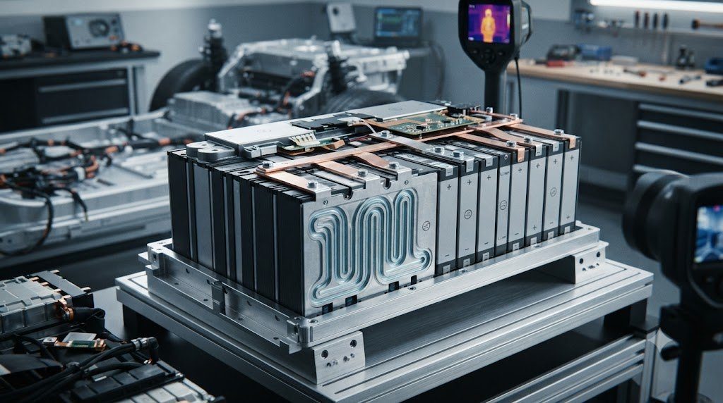
In any multi-cell lithium battery pack—whether powering an electric vehicle with 96 cells in series or a multi-megawatt grid energy storage container with thousands of interconnected cells—the entire pack is fundamentally constrained by its weakest single cell. Manufacturing variations in capacity, internal resistance, and self-discharge rates cause series-connected cells to diverge in voltage and State of Charge (SOC) over time. Without continuous cell balancing, the lowest-capacity cell limits pack discharge while the highest-voltage cell prematurely halts charging, stranding massive usable energy. Exploring passive resistive shunting versus active inductive, capacitive, and transformer-based energy redistribution reveals the critical control architecture of the modern Battery Management System (BMS).
The Weakest Link Principle in Battery Packs
In a series string of lithium-ion cells, charging must terminate the exact millisecond the most charged cell reaches its upper cutoff voltage (e.g., 4.20V) to prevent fire hazards. Conversely, discharging must terminate the moment the most depleted cell reaches its lower cutoff voltage (e.g., 2.80V) to avoid cell destruction. An un-balanced 100 kWh pack can see its usable capacity shrink to 60 kWh simply due to a 5% state-of-charge mismatch between two series cells.
1. Root Causes of Cell Imbalance: Production Variance and Thermal Gradients
Even when battery cells originate from the same production batch in an automated gigafactory, microscopic discrepancies are physically unavoidable:
- Active Material Coating Tolerances: Sub-micron variations in cathode slurry loading and electrode calendering produce initial manufacturing capacity mismatches of ±1.0% to 1.5% between individual cells.
- Electrolyte Degradation and Self-Discharge Divergence: Trace differences in SEI layer thickness and residual moisture cause varying chemical self-discharge rates. Over months of operation, a cell self-discharging at 2.5% per month will diverge significantly from a neighboring cell self-discharging at 1.5% per month.
- Pack Thermal Gradients (The Dominant Culprit): In real-world battery enclosures, cells positioned in the center of the module run 3°C to 7°C warmer than perimeter cells located next to external cooling ducts. According to the Arrhenius law, chemical aging rates double with every 10°C temperature increase. The warmer cells degrade faster, lose capacity quicker, and diverge irreversibly in internal impedance ($R_{int}$), permanently breaking series balance.
2. Passive Cell Balancing: Controlled Resistive Bleed Shunting
The overwhelming majority of commercial consumer electronics, power tools, and automotive battery packs utilize passive cell balancing due to its rock-solid reliability, low cost, and circuit simplicity:
Working Principle of Passive Bleed Resistors
In passive balancing, a small power resistor (typically 10 to 100 Ohms) is connected in parallel with every series cell, controlled by an electronic switch (MOSFET) governed by the BMS balancing IC:
- During the constant voltage (CV) stage of charging, the BMS monitors individual cell voltages via precision analog-to-digital converters (ADC).
- When a cell voltage rises above the balancing threshold (or exceeds the average string voltage by more than 10 to 15 millivolts), the BMS turns ON that cell’s MOSFET.
- Current is shunted through the parallel bleed resistor, dissipating excess energy as pure waste heat ($P = V^2 / R$) and bleeding down the higher cell until the remaining cells catch up.
Limitations of Passive Balancing
Passive balancing current is strictly thermally limited. Because dissipation resistors generate heat inside the tightly packed, sealed BMS circuit board, bleed currents are typically capped at only 50 mA to 200 mA. For a massive 100 Ah automotive or 300 Ah grid cell, a 100 mA balancing current would take dozens of hours to correct even a modest 2% state-of-charge mismatch!
| Balancing Metric / Attribute | Passive Balancing (Resistive Bleed) | Active Balancing (Switched Capacitor) | Active Balancing (Inductive / DC-DC) |
|---|---|---|---|
| Energy Handling | Dissipates excess energy as waste heat | Transfers energy between adjacent cells | Transfers energy cell-to-pack or cell-to-cell |
| Typical Balancing Current | 50 mA – 200 mA (Thermally limited) | 500 mA – 2.0 A (Moderate) | 1.0 A – 5.0+ A (High rate) |
| Energy Efficiency | 0% (All shunted energy lost) | 85% – 92% (Low transfer losses) | 88% – 95% (High DC-DC efficiency) |
| Circuit Complexity | Minimal (1 MOSFET + 1 resistor per cell) | Moderate (Array of switches + capacitors) | High (Inductors, transformers, isolated ICs) |
| BMS Hardware Cost | Very Low ($5 – $15 per pack) | Moderate ($30 – $75 per pack) | High ($100 – $300+ per pack) |
| Operational Regime | Active primarily during top-of-charge CV | Operates during charge, discharge, and rest | Operates continuously under any pack state |
| Dominant Use Case | Consumer EVs, power tools, home ESS | Heavy-duty electric trucks, commercial ESS | Aerospace, submarines, grid utility storage |
3. Active Cell Balancing: Non-Dissipative Energy Redistribution
Instead of burning off excess electrical charge as waste heat, active cell balancing physically shuttles energy from high-voltage cells to low-voltage cells, achieving near 90%+ energy efficiency:
Switched Capacitor (Charge Pump) Topologies
Switched-capacitor architectures utilize high-capacitance ceramic or electrolytic capacitors switched rapidly between adjacent series cells via MOSFET bridges:
- In Phase 1, the capacitor is connected across Cell $N$ (the higher-voltage cell), charging the capacitor to cell potential.
- In Phase 2, the MOSFET switch flips, connecting the charged capacitor across adjacent Cell $N-1$ (the lower-voltage cell), dumping charge into the depleted cell.
- By oscillating at frequencies between 10 kHz and 100 kHz, charge continuously “pumps” down the voltage gradient. While simple, transferring charge across a string of 96 cells requires multiple sequential hops, making end-to-end balancing slow.
Inductive and Isolated DC-DC Bidirectional Converters
The highest-performance active balancing systems employ bidirectional flyback transformers or multi-winding inductors:
- Cell-to-Pack Transfer: Excess energy from any high cell is energized into the primary inductor winding, stepped up in voltage, and injected back into the main high-voltage battery bus to charge the entire pack collectively.
- Pack-to-Cell Transfer: Energy is drawn from the bulk battery bus and stepped down directly into the single most depleted cell. This allows balancing currents upwards of 2.0A to 5.0A, enabling rapid dynamic balancing even while an electric vehicle is driving down the highway at 70 mph!
4. Balancing Strategies: Top Balancing vs. Bottom Balancing
The timing and reference point of balancing algorithms dictate whether battery packs prioritize maximum driving range or over-discharge safety:
- Top Balancing (Industry Standard for EVs): Balancing algorithms activate exclusively when cells reach the upper voltage knee (e.g., above 4.10V during charging). Top balancing guarantees that all cells reach 100% full saturation simultaneously, maximizing total usable energy storage and vehicle driving range on every full charge cycle.
- Bottom Balancing (Specialized Off-Grid / Racing): Balancing occurs at the bottom of the discharge curve when cells approach 2.80V. Bottom balancing ensures that all cells reach empty at the exact same instant, completely eliminating the danger of a weak cell reversing polarity or suffering catastrophic deep over-discharge under high-load acceleration. However, cells will have mismatched voltages at full charge.
5. The Voltage Measurement Challenge: LFP’s Ultra-Flat Voltage Plateau
While balancing NMC or NCA chemistries is straightforward because voltage correlates directly with state of charge (steep slope from 3.6V to 4.2V), Lithium Iron Phosphate (LFP) introduces an extreme measurement challenge:
Between 20% and 85% SOC, LFP’s open-circuit voltage sits on an almost mathematically flat plateau at 3.25V to 3.30V. A voltage change of merely 5 millivolts can correspond to a massive 30% difference in state of charge! If a BMS attempts to balance LFP cells in this flat mid-SOC zone based on voltage alone, measurement noise and minor load variations will cause the BMS to bleed the wrong cells. Consequently, LFP battery systems enforce balancing strictly above 3.45V per cell, where the voltage curve abruptly curves upward into a steep, unmistakable knee.
6. State-of-Charge (SOC) Estimation Algorithms: Coulomb Counting and Kalman Filters
Modern BMS balancing ICs do not rely solely on instantaneous raw voltage measurements; they execute sophisticated state estimation models:
- Coulomb Counting (Current Integration): Measures current in and out of the pack via precision high-side shunt resistors or Hall-effect sensors ($SOC(t) = SOC(0) – \int I(t) dt / Q_n$). However, sensor offset drift and round-off errors cause Coulomb counting to drift over time.
- Extended Kalman Filtering (EKF): Combines mathematical equivalent circuit models (ECM) with real-time voltage, current, and temperature measurements. The EKF recursively estimates true internal cell state of charge and internal resistance, dynamically filtering out measurement noise and providing balancing algorithms with precise true state metrics regardless of load transients.
7. Automotive Balancing Hardware: Analog Front-End (AFE) Architecture
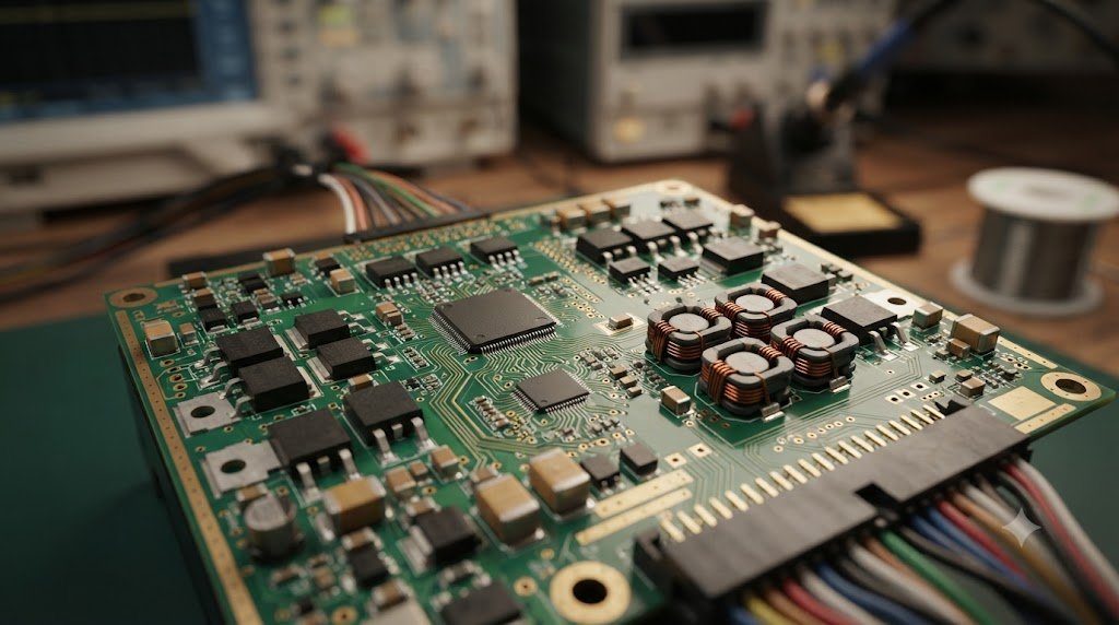
Translating balancing mathematics into hardware requires specialized automotive-qualified Analog Front-End (AFE) ICs (such as the Texas Instruments BQ79616 or Analog Devices LTC6813):
A single AFE IC monitors up to 16 to 18 series cells simultaneously with 16-bit delta-sigma ADCs achieving measurement accuracy better than ±1.5 millivolts across -40°C to +125°C. Internal MOSFET switches handle up to 200 mA of passive bleed current directly, with automatic fault detection that halts balancing if any thermal sensor detects resistor temperatures exceeding 85°C. Multiple AFE ICs daisy-chain via isolated differential SPI communications (isoSPI), delivering synchronized balancing commands across 800V battery packs.
8. Economic Comparison: Passive Bleeding vs. Active ROI in Utility Storage
In passenger electric vehicles, the small capacity gain of active balancing rarely justifies its 5x higher hardware cost. However, in multi-megawatt grid energy storage systems (BESS), the economic calculus flips completely:
In a 100 MWh utility storage facility operating daily energy arbitrage, rescuing 2% to 4% of stranded pack capacity through active balancing translates to thousands of additional megawatt-hours delivered over a 15-year lifecycle. The extra revenue generated from high-rate active balancing easily offsets the higher initial capital expenditure (CapEx) of active BMS hardware within 3 to 5 years of commercial grid operation.
9. Safety Protocols: Wire Harness Break and Thermal Runaway Prevention
Balancing circuits connect directly to high-energy battery terminals, creating unique electrical hazards if safety protocols fail:
- Open-Wire Detection: If a voltage sense wire snaps or vibrates loose during vehicle operation, the ADC input floats, potentially reading zero volts. An un-safeguarded BMS might interpret this as a dead short or attempt aggressive charging. Automotive AFEs inject micro-amp test currents into sense pins every second to detect broken wire impedance instantly.
- MOSFET Short-Circuit Protection: If a passive bleed MOSFET fails shorted, its associated bleed resistor would conduct continuously, draining the cell down to zero volts and causing copper dissolution. The BMS monitors balancing pin voltages during idle states to flag stuck-on MOSFETs immediately.
10. Frequently Asked Questions Regarding Cell Balancing
Why do series-connected battery cells become unbalanced over time?
Microscopic manufacturing variations in capacity, differing self-discharge rates, and uneven operating temperatures cause cells to charge and discharge at slightly different speeds.
What is the difference between passive and active cell balancing?
Passive balancing bleeds off excess energy from high cells as heat through resistors; active balancing redistributes energy from high cells to low cells using inductors or capacitors.
Why is passive balancing used in most electric cars instead of active?
Passive balancing is inexpensive, highly compact, and exceptionally reliable; the small energy saved by active balancing does not justify the higher cost and circuit complexity.
What is Top Balancing?
Balancing that occurs when cells approach the upper charging limit, ensuring all cells reach 100% full capacity at the exact same instant to maximize driving range.
Why is cell balancing especially difficult on LFP batteries?
LFP has an extremely flat voltage curve between 20% and 85% SOC; tiny voltage changes represent large capacity differences, making voltage-based balancing impossible except at the top knee.
What happens if a battery pack has no cell balancing system?
The weakest cell will limit discharge and the strongest will halt charge prematurely; over time, the usable capacity of the entire pack shrinks drastically and cells risk overcharge fires.
What is the typical balancing current in passive systems?
Around 50 mA to 200 mA, which is strictly limited by the amount of waste heat that circuit board resistors can safely dissipate.
Can active balancing work while the vehicle is driving?
Yes, high-current active inductive balancing can transfer energy between cells continuously during driving, charging, or rest.
What causes the most severe cell imbalance in automotive packs?
Uneven temperature distribution across the battery enclosure; cells running just 5°C warmer age twice as fast and drift significantly in resistance.
What is an Analog Front-End (AFE) IC?
A specialized automotive-grade chip that measures cell voltages with millivolt accuracy, monitors temperatures, and controls balancing switches.
What is Bottom Balancing and where is it used?
Balancing at the lowest discharge point so all cells reach empty simultaneously, commonly used in racing to protect cells from reverse-polarity damage.
Why do utility energy storage systems favor active balancing?
In multi-megawatt facilities, active balancing recovers millions of dollars of stranded energy over a 15-year lifespan, easily paying back the hardware cost.